Josephus Problem - Understanding the solution with Recursion

 Today we are going to discuss a very well-known and insightful problem - Josephus Problem. The solution we will discuss utilizes recursion. So, some underlying complexity of recursion will also be cleared.

The Story

The problem starts with a story. Yosef ben Matityahu, as Josephus was known to the Jews, was born in the Rome-occupied Jerusalem in 37 CE. He became a community leader and an army commander during the Roman invasion of Israel, which ultimately resulted in the destruction of the 2nd Beit Hamikdash. During his defense of the Galilee region, Josephus and his 40 Jewish soldiers were trapped in a fortress surrounded by the Roman army. They knew that capture was not an option, as they would be tortured and their bodies mutilated, so they decided that death was the only option. But, there was another problem. In Jewish law, it is better to kill someone than to commit suicide. So, together they devised a system where all the soldiers got in a circle, and each soldier killed his comrade to the left of him (in succession) until there would be one soldier left who would commit suicide. This plan would minimize the number of suicides in an organized manner, thereby solving their initial problems. However, Josephus had a different plan in mind: he wanted to survive and turn himself into the Romans. So, knowing that he couldn’t run away since his soldiers would turn on him, he had to calculate which place in the circle he had to be to survive this “circle of death.”

There were 41 people in the circle, and Josephus correctly calculated that to survive, he would have to be number 19. Josephus’ plan worked, and after turning himself in to the Romans, he became a famous historian by the name of Josephus Flavius and lived to tell this incredible story. Since then, this story has become a famous math problem. Many have wondered how Josephus knew which spot in the circle to be in and whether there is a formula to consistently determine which spot will survive given any number of people.

The Problem Statement

So, that's the problem to be solved. For a more generalized case, we would consider the number of soldiers is n, and each one would kill the one, who is k persons left to him. The problem statement without all the killing and with some sparkling of math will be something like:

We are given the natural numbers n and 
$k$. All natural numbers from$1$ to $n$ are written in a circle. First, count the k-th number starting from the first one and delete it. Then k numbers are counted starting from the next one, and the k -th one is removed again, and so on. The process stops when one number remains. It is required to find the last number.

Approaching the solution 

Let's assume a function, joseph, that gives us the person's position to be killed in the next turn. Our function joseph(n, k) would take the value of n and k as input. This function would internally utilize the killer's position to kill this next person, and that's where the recursion comes in. 

So, as the sword is passed to the next person of the last killed one. So we would get the next killer if we get the killed person of the last call, and add 1 to it, which would be something like the result from the previous call of the function +1, which should be the output of the next call.

 As we know, for most of the recursion problems, we have to take a base case. Let's take a case where n = 1. That means we are considering the beginning, where person 1 was the killer, thus the best case.

But who would have the first killer(person 1 ) killed? Obviously, the k-th next person to him,  person k. Again, if person 2 was the killer, who would he have killed? Person K+1 for sure.

Then how do we get the killed person from the position of the killer? 1 + (k-1) = k and 2 + (k-1) = k+1. Hmm...So adding (k-1) would do the trick. So until now, what we got is, our function will return the next person to be killed, so we would get the last standing person at the final call. And how will it predict the next to be killed? Somehow It will get the last killer. Add (k-1) to it to get the last killed person. And as the sword will be passed to the next person of the last killed person (who is also the next killer as he has the sword), we will find him out by adding 1 to the last killed person and return it as function output.

Feeling a little lost? Don't worry... the first time also happened to me when I thought about it. Just Take a deep breath.. and again read the last past. And now it would be more clear as we are going to write the pseudocode.

  
   function joseph (n, k) {
     return ( last killed person from last function call + (k-1) ) + 1
  }
  

Now just one problem. Look at the picture I provided. As there is no person after 6, the loop passes through the beginning of the array. Let me give an example. Suppose Person 6 was our next killer. Who is he going to kill? From the previous code we see, we will get person 8 as the killed one. As there is person 1 beside person 6, he would kill person 2 if it was his turn.

So we have to come back to the beginning after passing through the end. And who is better than modulus to do the task?

So the modified pseudocode will be, 

  
   function joseph (n, k) {
     return ( last killed person from last function call + (k-1) ) mod n + 1
  }
  

Great!! We are almost done, Just to figure out what the internal function call would be.  As every time a person gets killed, one person is reduced from the population(n-1), but the number of persons we jump over(k) remains constant.

The solution

the final recursive function to solve the Josephus problem, 

  
   function joseph (n, k) {
     return ( joseph(n-1, k) + (k-1) ) mod n + 1
  }
  

Not long ago , I have started reading object tracking publications. Soon I realized , this aspect of Computer Vision  has a lot of basic concepts and terms , that are different from Image classification or Object detection. So, I had to dig a lot. This post is to save the time that you were going to spend digging. 

We are going discuss about a lot of topics here.  SO, lets take an overview. 

• Main theme of object tracking
• Main components (Object Detection and Re-IDentification)
• Types and variations (Online vs. Offline, One Step vs Two Step, Anchor Based vs Anchor free)
• Famous Object tracking datasets
• State-of-the-art models
• Object tracking metrics

So, I hope you understand, This is going to be a long journey, I even may end up dividing it in two parts. So grab a coffe and lets jump in...

Main theme of object tracking

Object tracking has been a longstanding goal in computer vision. The goal is to estimate the trajectories of multiple objects of interest in videos. The successful resolution of the task can benefit many applications such as action recognition, sport videos analysis, elderly care, and human computer interaction.

Unlike image classification(which is considered to be one of the solved problem of CV, that's why the focus is moving to other fields , like 3D image classification), object tracking is considered to be an active research field of Computer vision. 

Just like we learn to walk before running, Our first goal in object tracking was tracking a single object in a video (Single Object Tracking - SOT) .

 As time passed, we moved to more complicated tasks, as a consequence, today we are mostly dealing with tracking multiple objects like cars, persons etc. (Multiple Object Tracking - MOT). 

Hopefully you can understand, this is considerably a difficult task than the previous one mentioned, as all persons and all cars look almost similar from a distance footage. 

Yet there are more problems. Often we see some objects are occluded from the footage, like a person  getting into a car or getting out of  a car. Besides, often the person or object moves so fast that its position changes considerably between two subsequent frames. So the model has to initiate or close a trajectory in the middle of a video footage. We are trying and also succeeding to overcome these and many other obstacled, and to make tracking computation and memory efficient.

Main components

In machine learning some problems are solvable in one shot, like image classification ( The total process can be completed only with one convolution network). Some are not, like Object detection(some network is used for extracting features from image, another for specifying the location of an object, some other for determining the best height and width for bounding the object with a box). One shot processes are faster, so researchers are finding methods to execute all the processes in single shot.

The main process of object tracking is divided into two tasks. Firstly detecting all objects in each frame of a video, and identifying a specific detection in each frame (actually only in those frames where that specific object is present) of that video.

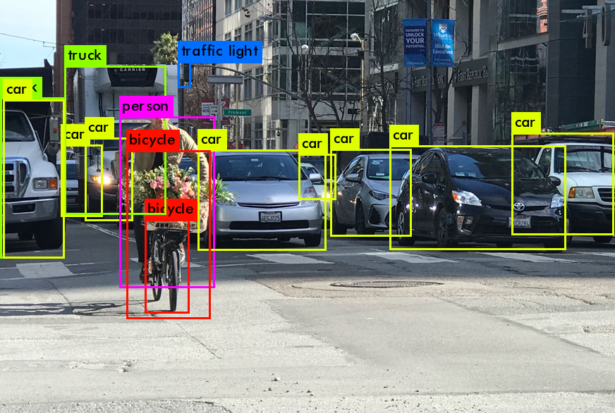
Object Detection: This part is simply detecting various objects in an image (frame of video), and drawing bounding box around that. This task is often done in two or three steps.Object detection , by itself is such a huge and evolving field of computer vision.Some of the best models for  this task are : YOLO(v1....v5), Faster R-CNN, SSD  and a lot others. But for now , were dont need to dive deeply here.

Re-ID: Now you must be thinking, isn't detection enough? Isn't out target detecting all objects trough all frames? Sadly no. We are yet to assign a detection to a specific object(ID), to track its  movement and finally finding the trajectory of that object (and similarly to every individual object in the video). That is the task of the process Re-IDentification, Identifying the same objects again and again in every frame.

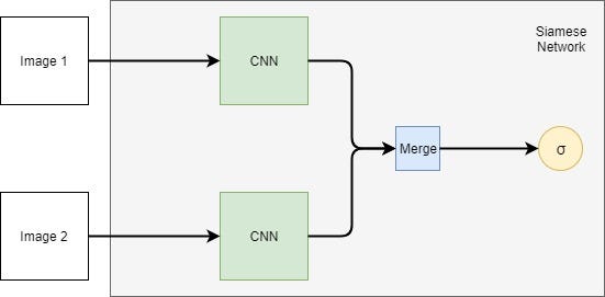
There has been a lot of work its improvement, yet we haven,t got the best of re-Identification. A vary populur approach for this is use of Seamese Network. Lets describe it briefly.HEre we usually train the model to learn similarity between two images. We will input two images to exactly same convolutional model, and the model is set to output the similarity score between those images. It will give a higher similarity score if those two input image represent the same object. Otherwise, low score. For efficient convergence, triplet loss or group loss are used as loss function.(Lets discus the loss functions some other day, but you can always google)Do you know, this is one of the most used algorithm for famous Face verification process, that we often encounter at ouur phone? and seamese network is cameble of learning with very small training dataset, that's why it is considers few shot learninig algorithm.

Types and variations

Like any other thing creation in this mortal world, object tracking algorithms also have a number of variations. Some variations are for making it fast, some changes make it computational cost efficient, and some  are just to be there. We will dis cuss about two or three important ones.

Online vs. Offline: Some tracking models are completely trained on stored dataset whereas some can be trained on live streaming footage. Both method has some advantages and some shortcomings.

Models that are suitable for training on live streaming video, are usually vary fast. Actually they are bound to be fast, otherwise it is impossible  to cope up with the video frame rate. of this speed, these models can be used for live object tracking. Some important online models are:

 

EfficientNet: A new approach to Neural Network scaling

Recently I came across a paper EfficientNet: Rethinking Model Scaling for Convolutional Neural Networks. They propose some amazing approach for scaling (increasing depth, width and resolution) neural network models. Here I will discuss the approach and try to build the intuition behind this approach. For mathematical and deeper insight, I recommend reading the original paper which is linked below.

You may have heard of EfficientNet as a image classification algorithm. Then why am I referring this as an approach, not an algorithm,which one is it? Lets find out!

First things first.Why EfficientNet? EfficientNet models (or approach) has gained new state of the art accuracy for 5 out of the 8 datasets,with  9.6 times fewer parameters on average.

At the paper, the authors firstly find out the relationship between the accuracy and the scaling(size) of a model.It is found that , performance increasing along with increase of width(number of channels used in each layer), depth(how many layers in the model)  and resolution(size of the input image).

We can see, at every case, initially the accuracy increases dramatically (of course along with the computational cost), but after sometime the curves almost flatten.

At this case, where depth is increased, everything else(width, resolution) is kept fixed. But the performance doesn't saturate so easily, if we increase all of them simultaneously and that's the first key observation in that paper.

Intuitively also, this makes a great sense. Because, for higher resolution image we can extract more features with a deeper neural network. Similarly, with increased width of the model, more fine grained  patterns can be captured from a higher number of pixels. From this we can sense that, co-ordination and balance between different scaling dimensions can help us achieve greater performance.

Generally this balance is tried to achieve by arbitrary change and manual tuning. But here we will take a more methodological approach. And this approach, compound scaling method is the second key observation of this paper.

Without getting into the mathematical details (for which I will recommend reading the original paper linked below), we can say that our authors have found a way , that if we increase the depth, width and height by a power of N,  our computation cost will increase by a power of 2 to the power N. And that is the compound scaling method.

By applying this concept and some nitty-gritty math details, authors first scaled up some existing state of the art ConvNets, like MobileNets and ResNets, which showed great improvement over their authentic performance, as well as their manually scaled versions.

Then ,they set out to a journey, for developing their own optimized model. By using some recently developed neural architecture search methods, at first a baseline model EfficientNet-B0 was created. Then it was scaled up by using previously discussed compound scaling method, developing the other versions, from EfficientNet-B1 to EfficientNet-B7. And that's what did the magic!!

Here is their performance on the ImageNet dataset compared with models of similar Top-1/Top-5 accuracy(If you aren't sure what the Top-1/Top-5 accuracy,  just take the Top-1 accuracy as the regular household accuracy,besides a little Google/Youtube search doesn't hurt).

And that's even not the whole story, the real magic is on the rightmost column.If  the term Flops is unknown,take that as number of total addition or multiplication operation needed for the process (again a little googling, you may search FLOPS vs FLOPs), actually it is the measure of computational power needed. And do you find something amazing?? 

Yap! So do I. The dramatic difference between EfficientNet models and their comparable models.Thing how much computationally efficient these EfficientNet models really are. Are they really comparable in those groups??

So, that's almost the story of one one the most powerful and scalable image classification models in recent years. Although a lot is left, like use of EfficientNet in transfer learning, as well as inference Latency comparison with other models. But lets leave that for your reading the paper.

Hope you get the main idea behind this amazing approach. Do you know , our EfficienNet has a detective brother, EfficientDet!! But that's a story for a different day.

Thanks for reading till here.You can read the original paper at https://arxiv.org/pdf/1905.11946

This is actually my first blog as well as first paper review. So, if you have any suggestions for me, I'm always open to them. Stay safe!!!